A brief Introduction to Support Vector Machine

Support Vector Machine (SVM) is one of the most popular Machine Learning Classifiers. It falls under the category of Supervised learning algorithms and uses the concept of Margin to classify between classes. It gives better accuracy than KNN, Decision Trees and Naive Bayes Classifier and hence is quite useful.

Who should read this post

Anyone with some prior knowledge of Machine Learning concepts and is Interested in learning about SVM. If you are a beginner in the field, go through this post first.

After reading this post, you’ll know:

1. What is SVM exactly
2. How to use SVM classifier from Sklearn (Python)
3. Tuning its parameters for better results

So let’s begin!

What is SVM?

As mentioned earlier, SVM lies in the class of supervised algorithms used for classification. Let’s start with a 2 class example:

Given classes X1 and X2, we want to find the decision boundary which separates the 2 classes the best i.e. with minimum error.

SVM does this with a ‘Hyperplane’. Now this hyperplane can be a single line in case of a 2-dimensional data and can be a plane in 3-dimensional one.

Without going into the math behind the curtain, let’s understand some basic functionality here.

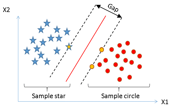
Support Vector Machines uses the concept of ‘Support Vectors‘ , which are the closest points to the hyperplane.

In the above example, the red line denotes our decision boundary that separates the 2 classes (Blue stars and Red circles) and the hyphened lines represent our ‘ Margin’ , the gap we want between the Support Vectors of both the classes.

Boundaries are Important

The Margin is defined with the help of the Support Vectors (hence the name). In our example, Yellow stars and Yellow circles are the Support Vectors defining the Margin. The better the gap, the better the classifier works. Hence support vectors play an important role in developing the classifier.

Every new data point in test data will be classified according to this Margin. If it lies on the right side of it, it’ll be classified as a Red circle otherwise as a Blue star.

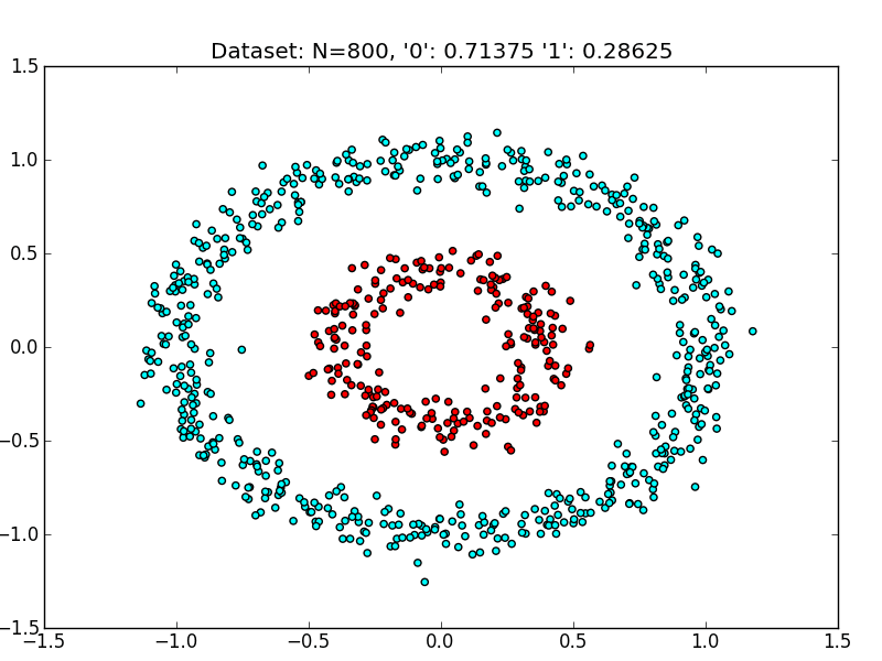
The best part is, SVM can also classify non-linear data.

Things get a little tricky in the case of non-linear data. Here SVM uses the ‘K_ernel-trick_‘ , it uses a kernel function to map the non-linear data to higher dimensions so that it becomes linear and finds the decision boundary there.

A Kernel function is always used by SVM, whether it is linear or non-linear data, but its main function comes into play when the data is inseparable in its current form. Here, the Kernel function adds dimensions to the problem for classification.

Now let’s see some code.

Using Support Vector Machines

With the help of Sklearn, you can harness the power of SVM classifier with just a few lines of code.

from sklearn import svm

#Our linear classifier
clf = svm.SVC(kernel='linear')

''' 
X\_train is your training data y\_train are the corresponding labels y\_pred are the predicted samples of the test data X\_test 
'''

#Training our classifier on the training set with labels
clf.fit(X\_train, y\_train)

#Predicting output on the Test set 
y\_pred = clf.predict(X\_test)

#Finding the Accuracy 
print("Accuracy:",metrics.accuracy\_score(y\_test, y\_pred))

In this case, we are using a linear kernel as you can see. Depending on the problem, you can use different types of Kernel functions:

• Linear
• Polynomial
• Radial Basis Function
• Gaussian
• Laplace

… and many more. Choosing the right kernel function is important for building the classifier. In the next section, we will tune the hyperparameters for our making our classifier even better.

You can access the complete code here.

If you’re bored, here’s a cute cat!

Tuning Parameters

Kernel : We have already discussed how important kernel functions are. Depending on the nature of the problem, the right kernel function has to be chosen as the kernel-function defines the hyperplane chosen for the problem. Here is a list of the most used Kernel functions.

Regularization : Ever heard of the term Overfitting? If you haven’t I think you should learn some basics from here. In SVM, to avoid overfitting, we choose a Soft Margin, instead of a Hard one i.e. we let some data points enter our margin intentionally (but we still penalize it) so that our classifier don’t overfit on our training sample. Here comes an important parameter Gamma (γ), which controls Overfitting in SVM. The higher the gamma, the higher the hyperplane tries to match the training data. Therefore, choosing an optimal gamma to avoid Overfitting as well as Underfitting is the key.

Error Penalty: Parameter C represents the error penalty for misclassification for SVM. It maintains the tradeoff between smoother hyperplane and misclassifications. As mentioned earlier, we do allow some misclassifications for avoiding overfitting of our classifier.

These are the most important parameters used for tuning the SVM classifier.

Overall SVM has many advantages as it provides high accuracy, has low complexity and also works quite well for non-linear data. The disadvantage being, it needs more training time compared to other algorithms such as Naive Bayes.

That is it for SVMs! If you have any questions, let me know in the comments.

Congratulations on making it to the end of the post!

Here’s a cookie for you

If you enjoyed this post, don’t forget to like!

Originally published at adityarohilla.com on November 2, 2018.