K-Nearest Neighbor algorithm

The concept of the k-nearest neighbor algorithm evolves from our day-to-day life and the pondering we make. The algorithm resembles the quote "Show me who your friends are and I’ll tell you who you are?", that is what K-NN is all about. To put it in layman’s terms, whenever we have brand new data to classify. We discover its k- nearest neighbors from the training data

Features of K-NN Algorithm

• K-NN is a non-parametric algorithm which means it does not make any prediction on underlying data.

• It does not immediately learn from the training set as it stores the dataset at the time of classification and then performs an action on the set. Hence it is called as lazy learning algorithm.

Applications of K-NN Algorithm

• The largest application of the K-NN classifier might be the Recommendation system. If you know a user likes a particular product then you can recommend similar products for them.

• Credit ratings -By using K-NN we can calculate the credit ratings of a particular customer.

• Image recognition and Video recognition.

• Handwriting detection (like OCR)

Working of K-NN Algorithm

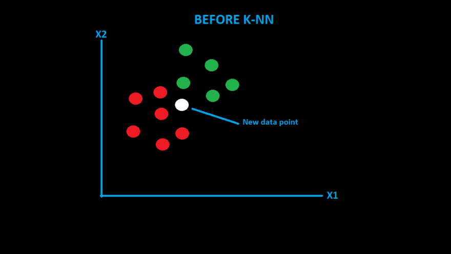
Let me explain with the assistance of an example. So that we can understand it easily. As you can see we have two categories which are red and green.

If we get a new datapoint, how would we categorize it? Let's find it through the K-NN algorithm.

1. the first step is to choose the value of K, by default it is 5.
2. Take the K-nearest neighbors of the new data point according to a distance algorithm and the most preferred is euclidian distance as it is the most popular one. if P1(x1,y1) are the coordinates of the new data point and P2(x2,y2) are the coordinates of the data points in Category-1 and Category-2 then the euclidian distance would be
3. Among the neighbors, count the number of data points in each category.
4. you can see most of the neighbors are from the red group. So our new data point would be categorized as the same.

Implementing K-NN Algorithm in python

We will be using the library sklearn for preprocessing and training the dataset.

import pandas as pd
url = "https://archive.ics.uci.edu/ml/machine-learning-databases/iris/iris.data"
column_names = ['sepal-length-cm', 'sepal-width-cm', 'petal-length-cm', 'petal-width-cm', 'Class']
data_set = pd.read_csv(url, names=column_names)

Here what we have done is we just imported library called pandas for fitting the dataset and then imported the famous iris dataset for the implementation.
Let us print the dataset.

We have the dataset now. The next step is to preprocess the data for making it suitable for model creation, for that we need to divide the dataset into independent and dependent variables. Here you can see that column 'Class' is the independent variable and the remaining things are features. Let us do that.

features = dataset.iloc[:, :-1].values
test_label = dataset.iloc[:, 4].values

Please understand that variable features would be having all the rows except column "Class" and test_label contains all the rows of column "Class".

Now we need to divide the data set into training and test dataset. We should be careful in this step as we should avoid both overfitting and underfitting for better results . Here we would be taking 80:20 ratio. This means that 80% of the dataset would be used for training the modal and the remaining 20% would be used for testing the created model.

from sklearn.model_selection import train_test_split
X_train, X_test, y_train, y_test = train_test_split(features, test_label, test_size=0.20)

We have divided the whole dataset into a training dataset and a test dataset. Machine learning algorithms work better when features are on a relatively similar scale. So we are going to use the standard scaler method from sklearn for preprocessing the dataset.

from sklearn.preprocessing import StandardScaler
scaler = StandardScaler()
scaler.fit(X_train) # 

X_train = scaler.transform(X_train)
X_test = scaler.transform(X_test)

Let us see the form of the data stored in X_train.

Now let us train the model. We will be using a built-in K-NN classifier for model creation.

from sklearn.neighbors import KNeighborsClassifier
classifier = KNeighborsClassifier(n_neighbors=5)
classifier.fit(X_train, y_train)
y_pred = classifier.predict(X_test)

We selected the K value as 5 . This means it will find 5 training examples that are closest to the new example and then assigns the test example to the most common class label (among those k-training examples).

Let us check the confusion matrix and accuracy for determining the efficiency of our model.

from sklearn.metrics import classification_report, confusion_matrix,accuracy_score
print(confusion_matrix(y_test, y_pred))
print(classification_report(y_test, y_pred))

As you can see we received a excellent precision and recall values. This means almost every positive sample are correctly detected.
We can also check the overall accuracy of the model.

acc = accuracy_score(y_test, y_pred)

We got almost 94 % accuracy . So our model performs well for the given test data.

Disadvantages of K-NN

• It would not work well if the dataset is very large.
• Does not work well with high measurements: So We need to reduce the measurements to tackle the problem, but it might not work in every case.
• Sensitive to noisy data: KNN is very sensitive to noise in the dataset , which will affect the overall result.
• It is expensive — because the algorithm stores all of the training data. So it uses a lot of memory.
• High memory requirement.

Conclusion
The k-nearest neighbors (KNN) algorithm is an effortless, supervised machine learning algorithm that can solve both classification and regression problems. But when the dataset becomes larger, the efficiency or speed of the algorithm would be compromised.

References:
K-NN algorithm, a short tour by krish naik

Disclaimer: This is a personal [blog, post, statement, opinion]. The views and opinions expressed here are only those of the author and do not represent those of any organization or any individual with whom the author may be associated, professionally or personally.