An in-depth technical dive into automating satellite data workflows, tackling real-world issues, and making your pipeline production-ready.
Introduction: Automating Satellite Data for Vegetation Monitoring
Monitoring vegetation health is essential for sustainable agriculture, environmental conservation, and understanding climate change impacts. One of the most trusted indicators is the Normalized Difference Vegetation Index (NDVI), which offers a quantifiable measure of vegetation vigor.
But working with raw satellite data is not straightforward.
In this article, I'll walk you through building an end-to-end, automated NDVI pipeline that:
✅ Downloads VIIRS NDVI data from Google Earth Engine (GEE).
✅ Cleans and clips the rasters to your region of interest.
✅ Aggregates the data monthly for time-series analysis.
✅ Resamples rasters to ensure uniform resolution.
✅ Converts the processed rasters to scientific NetCDF format.
✅ Orchestrates everything using Apache Airflow running on WSL (Windows Subsystem for Linux).
Along the way, I'll show you code snippets, architectural decisions, lessons learned (especially about Airflow persistence), and best practices such as ensuring resilience across machine restarts and terminal closures.
🧩 Tech Stack Overview
| Tool | Purpose |
|---|---|
| Google Earth Engine (GEE) | Access VIIRS NDVI dataset |
| Python | Data processing and automation |
| Rasterio & GDAL | Raster data manipulation |
| xarray & NetCDF4 | Multi-dimensional data handling and conversion to NetCDF |
| Apache Airflow | Pipeline orchestration and scheduling |
| WSL (Ubuntu on Windows) | Development environment |
| Systemd / nohup | Persistent service management |
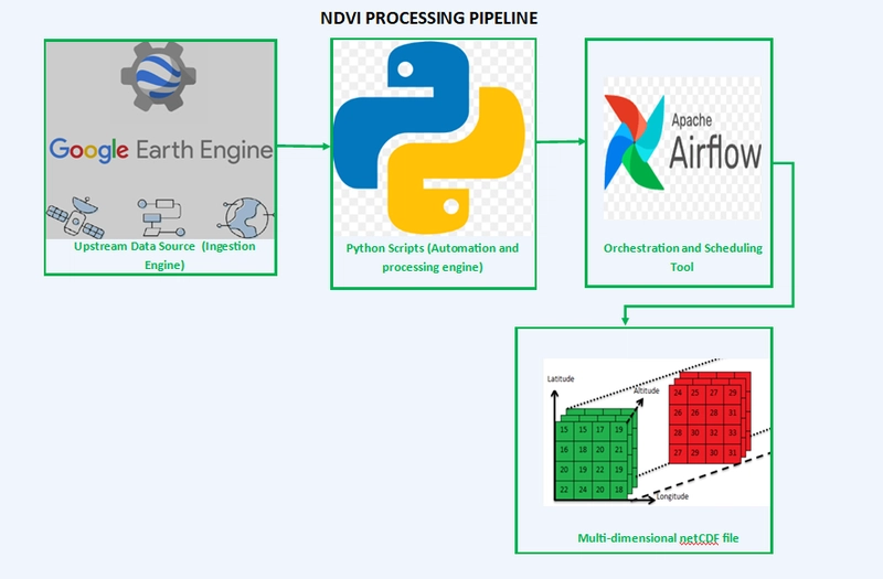
🔧 System Architecture
Google Earth Engine (GEE VIIRS)
           |
           v
Python Scripts (EE API)
           |
           v
Raw NDVI GeoTIFFs (local storage)
           |
           v
Airflow DAG (orchestration)
  |- Pre-processing: Clean & Clip Raster
  |- Monthly Aggregation
  |- Resampling
  |- Convert to NetCDF
           |
           v
Processed NDVI NetCDF outputs
Each step includes file existence checks to avoid redundant processing and ensure idempotency.
🛰️ Step 1: Download NDVI Data from Google Earth Engine
Using the GEE Python API, we query and download NDVI VIIRS data for our region of interest.
import ee

ee.Initialize()

def download_ndvi(start_date, end_date, region):
    collection = ee.ImageCollection('NOAA/VIIRS/001/VNP13A1')\
        .filterDate(start_date, end_date)\
        .filterBounds(region)

    for image in collection.getInfo()['features']:
        export_image(image, region)

# export_image implementation uses ee.batch.Export.image.toDrive or toCloudStorage
Best practice:
✔️ Set up service account authentication for seamless automation.
✔️ Ensure quotas are managed as GEE enforces limits.
✔️ Always check if the data already exists locally to avoid unnecessary downloads.
✔️ Log each operation for traceability.
🧹 Step 2: Cleaning and Clipping Raster Files
We clean the raw downloaded rasters and clip them to our specific area of interest. We checked if the data is missing in a pixel; if there is missing data, we filled the gap with the value of the nearest pixel. Why nearest pixel filling? (Tobler's first law of geography answers this.). Before processing, we check if the cleaned file already exists.
from rasterio.mask import mask
import rasterio

def clean_and_clip_raster(input_path, output_path, geojson):
    if os.path.exists(output_path):
        print("Clipped raster already exists.")
        return

    with rasterio.open(input_path) as src:
        with open(geojson) as f:
            shapes = [json.load(f)]

        out_image, out_transform = mask(src, shapes, crop=True)

        out_meta = src.meta.copy()
        out_meta.update({"driver": "GTiff",
                         "height": out_image.shape[1],
                         "width": out_image.shape[2],
                         "transform": out_transform})

        with rasterio.open(output_path, "w", **out_meta) as dest:
            dest.write(out_image)
Tip:
✔️ Add file existence checks at this step to skip already processed files.
📆 Step 3: Monthly Aggregation
Once cleaned, rasters are aggregated monthly using temporal grouping and mean calculations.
import numpy as np
import rasterio

def aggregate_monthly(file_list, output_path):
    if os.path.exists(output_path):
        print("Monthly aggregated raster already exists.")
        return

    arrays = [rasterio.open(f).read(1) for f in file_list]
    mean_array = np.nanmean(arrays, axis=0)

    meta = rasterio.open(file_list[0]).meta
    with rasterio.open(output_path, "w", **meta) as dest:
        dest.write(mean_array, 1)
✔️ File checks before processing
✔️ Exception handling in case rasters are missing
🔄 Step 4: Resample for Uniform Resolution
To ensure all rasters are at the same resolution, we resample them.
from rasterio.enums import Resampling

def resample_raster(input_path, output_path, scale):
    if os.path.exists(output_path):
        print("Resampled raster already exists.")
        return

    with rasterio.open(input_path) as dataset:
        data = dataset.read(1, resampling=Resampling.bilinear)
        transform = dataset.transform * dataset.transform.scale(
            (dataset.width / scale[0]),
            (dataset.height / scale[1])
        )

        profile = dataset.profile
        profile.update(transform=transform, width=scale[0], height=scale[1])

        with rasterio.open(output_path, "w", **profile) as dst:
            dst.write(data, 1)
🌐 Step 5: Convert to NetCDF
The final rasters are converted into a scientific format (NetCDF). We use xarray and netCDF4 to convert to a scientific, multi-dimensional format.
import xarray as xr

def convert_to_netcdf(input_path, output_path):
    if os.path.exists(output_path):
        print("NetCDF file already exists.")
        return

    raster = rasterio.open(input_path)
    data = raster.read(1)

    ds = xr.Dataset(
        {'NDVI': (['y', 'x'], data)},
        coords={'y': np.arange(data.shape[0]), 'x': np.arange(data.shape[1])}
    )

    ds.to_netcdf(output_path)
✔️ Ensures scientific usability.
✔️ Compact and efficient storage
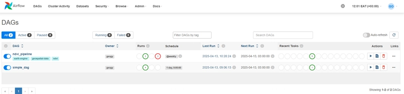
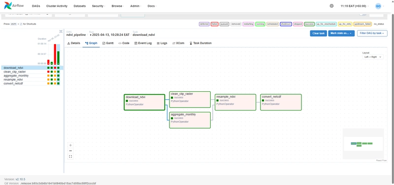
🚀 Orchestrating with Apache Airflow on WSL
Here’s an Airflow DAG that orchestrates everything:
from airflow import DAG
from airflow.operators.python import PythonOperator
from datetime import datetime

def pipeline():
    download_ndvi(...)
    clean_and_clip_raster(...)
    aggregate_monthly(...)
    resample_raster(...)
    convert_to_netcdf(...)

def build_dag():
    with DAG('ndvi_pipeline', start_date=datetime(2025, 4, 1), schedule_interval='@monthly', catchup=False) as dag:
        task = PythonOperator(task_id='run_pipeline', python_callable=pipeline)
        task
    return dag

dag = build_dag()
✔️ Automates the entire flow.
✔️ Airflow handles scheduling, retries, and logs.
🖥️ Keeping Airflow Running (WSL Tips)
One challenge with WSL is Airflow stopping after closing your terminal or sleeping your computer.
Solution 1: Use nohup
Run airflow services in the background:
nohup airflow webserver --port 8080 > ~/airflow-webserver.log 2>&1 &
nohup airflow scheduler > ~/airflow-scheduler.log 2>&1 &
Solution 2: Set up systemd for automatic service management.
Airflow Debugging Tips:
- Always check
airflow-webserver.logandairflow-scheduler.logfor real-time errors. - Ensure your DAG is being picked up:
airflow dags list - If "scheduler heartbeat" warnings appear, restart your scheduler!
🧩 Best Practices
- ✅ File existence checks: Avoid redundant processing.
- ✅ Robust logging: Add logging at every step for easier debugging.
- ✅ Airflow retries: Configure retries in your DAG for network hiccups.
- ✅ Environment isolation: Use
virtualenvin WSL to avoid dependency issues. - ✅ Backup workflows: Regularly export Airflow DAGs and environment configs.
🌟 Final Thoughts
What started as a fragmented manual process is now a robust, automated, and maintainable pipeline. From fetching raw satellite data to delivering ready-to-use NetCDF files, this system enables repeatable workflows for vegetation analysis at scale. This pipeline is scalable, reliable, and fully automated. Whether you're monitoring agricultural fields or researching climate impacts, this setup ensures you always have clean, processed, and usable data at your fingertips.
If you'd like, I can also share:
- 📂 My full repository (Python scripts + DAGs.
- 🎥 Video demo of the pipeline.
- 📊 Dashboarding suggestions for visualizing NDVI over time!
This isn’t just an NDVI pipeline — it's a blueprint for any geospatial ETL (Extract, Transform, Load) process.
Next Steps:
- Add alerting (Slack or Email) for failed tasks.
- Containerize the pipeline with Docker.
- Schedule nightly or real-time updates.
- Visualize outputs with dashboards (Grafana or Plotly Dash).
Let’s connect! 🚀
🐙 GitHub
💼 LinkedIn
✖️ X (Twitter)
If you enjoyed this article, feel free to follow me for more articles on geospatial data science, data engineering, automation, and efficient scientific workflows! 🚀 Drop your comments in the comment section below.
Written by George Odero, Geospatial Data Engineer & Automation Enthusiast.

Top comments (1)
Hi George,
I would really appreciate it if you could share the repository for this project, it would be a great resource for learning how to use raster data with AirFlow
Greetings!