When you have large volumes of data, storing it logically helps users discover information and makes understanding the information easier. In this post, we talk about some of the techniques we use to do so in our application.

In this post, we are going to use the terminology of AWS S3 buckets to store information. The same techniques can be applied on other cloud, non cloud providers and bare metal servers. Most setups will include a high bandwidth low latency network attached storage with proximity to the processing cluster or disks on HDFS if the entire platform uses HDFS. Your mileage may vary based on your team’s setup and use case. We are also going to talk about techniques which have allowed us to efficiently process this information using Apache Spark as our processing engine. Similar techniques are available for other data processing engines.

Managing storage on disk

When you have large volumes of data, we have found it useful to separate data that comes in from the upstream providers (if any) from any insights we process and produce. This allows us to segregate access (different parts have different PII classifications) and apply different retention policies.

We would separate each of these datasets so it’s clear where each came from. When setting up the location to store your data, refer to local laws (like GDPR) for details on data residency requirements.

Provider buckets

Providers tend to make their own directories to send us data. This allows them to have access over how long they want to retain data or if they need to modify information. Data is rarely modified but when it is, a heads up is given to re-process information.

If this was an event driven system, we would have different event types suggesting that the data from an earlier date was modified. Since the volume of data is large and the batch nature of data transfer on our platform, verbal/written communication is preferred by our data providers which allows us to re-trigger our data pipelines for the affected days.

Landing bucket

Most data platforms either procure data or produce it internally. The usual mechanism is for a provider to write data into its own bucket and give its consumers (our platform) access. We copy the data into a landing bucket. This data is a full replica of what the provider gives us without any processing. Keeping data we received from the provider separate from data we process and insights we derive allows us to

1. Ensure that we don’t accidentally share raw data with others (we are contractually obligated not to share source data)
2. Apply different access policies to raw data when it contains any PII
3. Preserve an untouched copy of the source if we ever have to re-process the data (providers delete data from their bucket within a month or so)

Core bucket

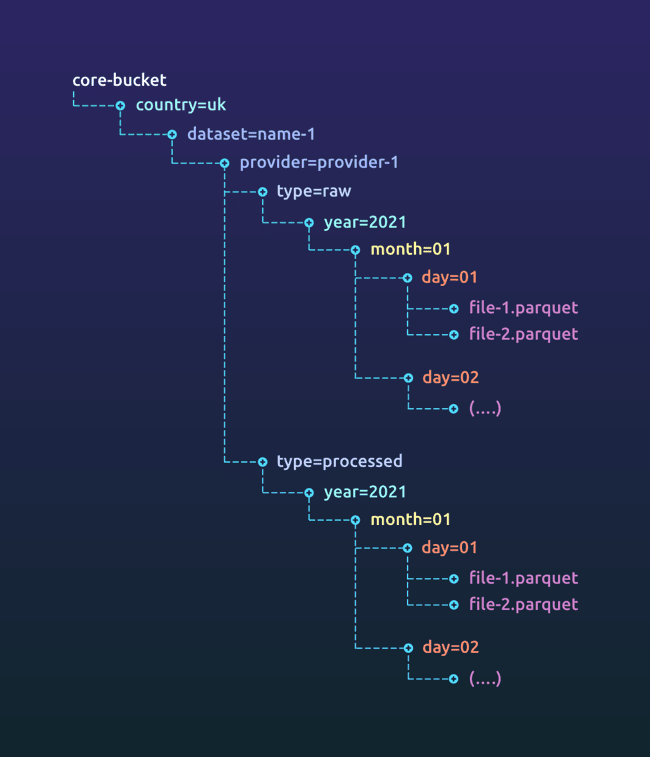
The data in the landing bucket might be in a format sub optimal for processing (like CSV). The data might also be dirty. We take this opportunity to clean up the data and change the format to something more suitable for processing. For our use case, a downstream pipeline usually consumes a part of what the upstream pipeline produces. Since only a subset of the data is read downstream by a single job, using a file format that allows optimized columnar reads helped us boost performance and thus we use formats like ORC and parquet in our system. The output after this cleanup and transformation is written to the core bucket (since this data is clean input that’s optimised for further processing and thus core to the functioning of the platform).

While landing has an exact replica of what the data provider gave us, core’s raw data just transforms it to a more appropriate format (parquet/ORC for our use case) and processing applies some data cleanup strategies, adds meta-data and a few processed columns.

Derived bucket

Your data platform probably has multiple models running on top of the core data that produce multiple insights. We write the output for each of these into its own directory.

Advantages of data segregation

1. Separating the data makes it easier to find the data. When you have terabytes or petabytes of information across your organisation with multiple teams working on this data platform, it becomes easy to lose track of the information that is already available and it can be hard to find it if they are stored in different places. Having some way to find information is helpful. For us, separating the data by whether we get it from an upstream system, we produce it or we send it out to a downstream system helps teams find information easily.
2. Different rules apply to different datasets. You might be obligated to delete data from raw information you have purchased under certain conditions (like when they have PII). Rules for retaining derived data are different if it does not contain any PII.
3. Most platforms allow archiving of data. Separating the dataset makes it easier to archive different datasets. (we’ll talk about other aspects of archiving during data partitioning)

Data partitioning

Partitioning is a technique that allows your processing engine (like Spark) to read data more efficiently thus making the program more efficient. The most optimal way to partition data is based on the way it is read, written and/or processed. Since most data is written once and read multiple times, optimising a dataset for reads makes sense.

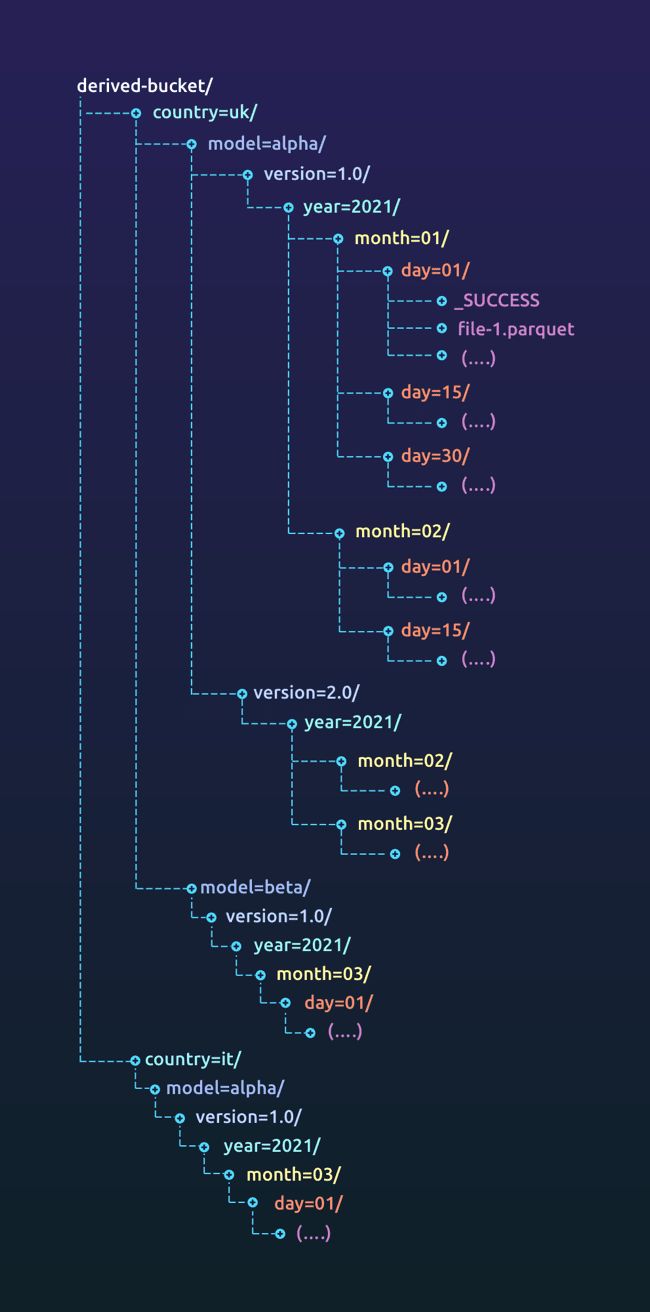
We create a core bucket for each region we operate in (based on data residency laws of the area). For example, since the EU data cannot leave the EU, we create a derived-bucket in one of the regions in the EU. Under this bucket, we separate the data based on the country, the model that’s producing the data, a version of the data (based on its schema) and the date partition based on which the data was created.

Reading data from a path like derived-bucket/country=uk/model=alpha/version=1.0 will give you a data set with columns year, month and day. This is useful when you are looking for data across different dates. When filtering the data based on a certain month, frameworks like spark allow the use of push down predicates making reads more efficient.

Data versioning

We change the version of the data every time there is a breaking change. Our versioning strategy is similar to the one talked about in the book for Database Refactoring with a few changes for scale. The book talks about many types of refactoring and the column rename is a common and interesting use case.

Since the data volume is comparatively low in databases (megabytes to gigabytes), migrating everything to the latest schema is (comparatively) inexpensive. It is important to make sure the application is usable at all points and that there is no point at which the application is not usable.

Versioning on large data sets

When the data volume is high (think terabytes to petabytes), running migrations like this is a very expensive process in terms of the time and resources taken. Also, the application downtime during the migration is large or there’s 2 copies of the dataset created (which makes storage more expensive).

Non breaking schema changes

Let’s say you have a dataset that maps the real names to superhero names that you have written to model=superhero-identities/year=2021/month=05/day=01.

+--------------+-----------------+
|  real_name   | superhero_name  |
+--------------+-----------------+
| Tony Stark   | Iron Man        |
| Steve Rogers | Captain America |
+--------------+-----------------+

The next day, if you would like to add their home location, you can write the following data set to the directory day=02.

+------------------+----------------+--------------------------+
|    real_name     | superhero_name |      home_location       |
+------------------+----------------+--------------------------+
| Bruce Banner     | Hulk           | Dayton, Ohio             |
| Natasha Romanoff | Black Widow    | Stalingrad, Soviet Union |
+------------------+----------------+--------------------------+

Soon after, you realize that storing the real name is too risky. The data you have already published was public knowledge but moving forward, you would like to stop publishing real names. Thus on day=03, you remove the real_name column.

+----------------+---------------------------+
| superhero_name |       home_location       |
+----------------+---------------------------+
| Spider-Man     | Queens, New York          |
| Ant-Man        | San Francisco, California |
+----------------+---------------------------+

When you read derived-bucket/country=uk/model=superhero-identities/ using spark, the framework will read the first schema and use it to read the entire dataset. As a result, you do not see the new home_location column.

scala> spark.read.
  parquet("model=superhero-identities").
  show()
+----------------+---------------+----+-----+---+
|       real_name| superhero_name|year|month|day|
+----------------+---------------+----+-----+---+
|Natasha Romanoff|    Black Widow|2021|    5|  2|
|    Bruce Banner|           Hulk|2021|    5|  2|
|            null|        Ant-Man|2021|    5|  3|
|            null|     Spider-Man|2021|    5|  3|
|    Steve Rogers|Captain America|2021|    5|  1|
|      Tony Stark|       Iron Man|2021|    5|  1|
+----------------+---------------+----+-----+---+

Asking Spark to merge the schema for you shows all columns (with missing values shown as null)

scala> spark.read.option("mergeSchema", "true").
  parquet("model=superhero-identities").
  show()
+----------------+---------------+--------------------+----+-----+---+
|       real_name| superhero_name|       home_location|year|month|day|
+----------------+---------------+--------------------+----+-----+---+
|Natasha Romanoff|    Black Widow|Stalingrad, Sovie...|2021|    5|  2|
|    Bruce Banner|           Hulk|        Dayton, Ohio|2021|    5|  2|
|            null|        Ant-Man|San Francisco, Ca...|2021|    5|  3|
|            null|     Spider-Man|    Queens, New York|2021|    5|  3|
|    Steve Rogers|Captain America|                null|2021|    5|  1|
|      Tony Stark|       Iron Man|                null|2021|    5|  1|
+----------------+---------------+--------------------+----+-----+---+

As your model’s schema evolves, using features like merge schema allows you to read the available data across various partitions and then process it. While we have showcased spark’s abilities to merge schemas for parquet files, such capabilities are also available with other file formats.

Breaking changes or parallel runs

Sometimes, you evolve and improve your model. It is useful to do parallel runs and compare the result to verify that it is indeed better before the business switches to use the newer version.

In such cases we bump up the version of the solution. Let’s assume job alpha v1.0.36 writes to the directory derived-bucket/country=uk/model=alpha/version=1.0. When we have a newer version of the model (that either has a very different schema or has to be run in parallel), we bump the version of the job (and the location it writes to) to 2.0 making the job alpha v2.0.0 and it’s output directory derived-bucket/country=uk/model=alpha/version=2.0.

If this change was made and deployed on 1st of Feb and this job runs daily, the latest date partition under model=alpha/version=1.0 will be year=2020/month=01/day=31. From the 1st of Feb, all data will be written to the model=alpha/version=2.0 directory. If the data in version 2.0 is not sufficient for the business on 1st Feb, we either run backfill jobs to get more data under this partition or we run both version 1 and 2 until version 2’s data is ready to be used by the business.

The version on disk represents the version of the schema and can be matched up with the versioning of the artifact when using Semantic Versioning.

Advantages

1. Each version partition on disk has the same schema (making reads easier)
2. Downstream systems can choose when to migrate from one version to another
3. A new version can be tested out without affecting the existing data pipeline chain

Summary

Applications, system architecture and your data always evolve. Your decisions in how you store and access your data affect your system’s ability to evolve. Using techniques like versioning and partitioning helps your system continue to evolve with minimal overhead cost. Thus, we recommend integrating these techniques into your product at its inception so the team has a strong foundation to build upon.

Thanks to Sanjoy, Anay Sathish, Jayant and Priyank for their draft reviews and early feedback. Thanks to Niki for using her artwork wizardry skills.