In this blog I will explain the functionality of this program, the purpose of this program is to iterate all the matrix adding the neighbor numbers, dividing it by the number of neighbors and put the result in the second matrix where the operation took place in the first matrix.
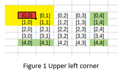
First of all, we’ll start in the Figure 1,As we can see the algorithm take place in the first matrix’s cell in color red, we can see that the matrix in the left side, upper left corner, and upper left side in color yellow doesn’t have neighbors, so the algorithm will take the opposite side, that is to say the cell in color green. The algorithm will save the result in the second matrix in the same position in color red.
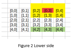
In the Figure 2, As we mention before, the algorithm will iterate through all the cells, in this case we can see that the algorithm had iterated through the cell [0,3],but we can see that the matrix doesn’t have the upper side neighbors in color yellow, therefore the algorithm will take the lower sides in color green, and the result will be adding in the second matrix in the same position in color red.
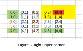
In the Figure 3, The algorithm takes the right upper corner in color red, but the matrix doesn’t have the neighbors in color yellow, Therefore, the algorithm takes the cells in color green, and the result will be adding in the second matrix in the same position in color red.
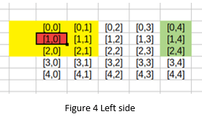
In the Figure 4,The algorithm had iterated until cell [1,0], but the matrix doesn’t have the neighbors in the left side in color yellow, Therefore, the algorithm will take the opposite side in color green, and the result will be adding in the second matrix in the same position in color red.
In the Figure 5, we can see that the algorithm takes the cell [1,1], and the matrix knows all its neighbors, which there’s no problem to do the operation.
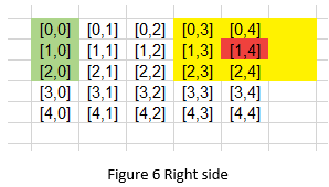
In the Figure 6, We can see that the algorithm had iterated through cell [1,4], but the matrix doesn’t have the neighbors in the right side in color yellow, whereby the algorithm will take the opposite sides in color green, and the result will be adding in the second matrix in the same position in color red.
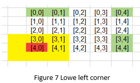
In the Figure 7, We can observe that in the cell in color red, it’s on the lower left corner and the matrix doesn’t have the neighbors in color yellow, whereby the algorithm will take the opposite sides in color green, and the result will be adding in the second matrix in the same position in color red.
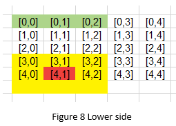
In the Figure 8, We can observe that the algorithm had iterated through the cell [4,1], but the matrix doesn’t have the neighbors in the lower side in color yellow, whereby the algorithm will take the opposite sides in color green, and the result will be adding in the second matrix in the same position in color red.
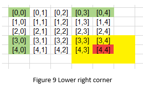
In the Figure 9,We can appreciate that the algorithm had reached to the last cell of the matrix in color red, but the matrix doesn’t have the neighbors in color yellow, whereby the algorithm will take the opposite sides in color green, and the result will be adding in the second matrix in the same position in color red.
Therefore, every figure is a technique and it will get in operation when the matrix doesn’t know its neighbors.
The code:
https://github.com/martincorona007/Graphics/tree/master/Program%202%20Matrix%20Circular





Top comments (0)