Update! You can find Part 2, where we explore coordinate frames for 3D systems, here.
Multi-sensor systems are becoming ever more common as we seek to automate robotics, navigation, or create a "smart" world. Any random assortment of sensors could be sensing any number of quantities, from barometric pressure, to temperature, to even more complex sensors that scan the world around us and produce 3D maps (like LiDAR). These multi-sensor systems often carry a great deal of complexity, to be able to learn about the world to the same degree that we can just by listening, feeling, and seeing our environment.
An important aspect of multi-sensor systems is how we relate these assorted sensing platforms together. If we are reading temperature, how do we use that value to make decisions? If we have multiple cameras, how can we tell if an object moves from the view of one camera to the next? Individual sensors on their own may be insufficient for making decisions, and therefore need to be linked together. There are a handful of ways we can correlate data, but one of the most powerful ways is to do so spatially. In this post, we're going to explore some of the language and tools we use for doing so.
Location, location, location
It's all about location. No, really. All sensors have some spatial property, and it is by relating sensors together in this way that we can produce useful results! Knowing that a sensor measured 30° C isn't particularly useful on its own. Knowing that a sensor in your thermostat measured 30° C is a much more useful distinction. The same holds true for more sophisticated sensors such as cameras, LiDAR, accelerometers, etc. These "advanced" sensors are even measuring spatial quantities, which are the backbone of modern robotics and automation.
Many of the useful aspects of multi-sensor systems are derived by a spatial understanding of the world around us. Location helps us decide how related any two quantities might be; rather, it is in relating things spatially that our sensors can derive the context of the world around us. Many of the problems in integrating new sensors into a robotics or automation system are therefore coordinate system problems. To understand this, we first need to talk about coordinate frames and then discuss how to relate any two coordinate frames.
Sensors and coordinate frames
A coordinate frame or coordinate system is a way for us to label the positions of some points using a set of coordinates, relative to the system's origin. A common type of coordinate frame is a Cartesian coordinate frame, which labels positions along a set of perpendicular axes. Consider the following Cartesian grid, defining a coordinate frame:
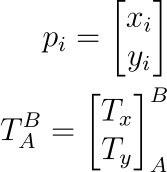
For a Cartesian frame, we denote the position of our points as a tuple with the offset from the origin O along each of the axes. In the above example, our point p has a coordinate of (2, 2), while q has a coordinate of (3, 4). For any point in the system, you can describe its coordinate as (xp, yp) for a point p, where xp is the offset from the origin O along the direction of the x-axis and yp is the offset from the origin O along the direction of the y-axis.
Other types of coordinate frames exist as well, including polar coordinate systems and spherical coordinate systems. Map projections such as Mercator or Gnomonic maps are also a type of projected coordinate system, that exist as a handy way to plot and interpret the same data in different ways. For now however, we will focus on Cartesian coordinate frames, as they tend to be the most commonly used coordinate frame to represent and interpret spatial data.
From the example above, we can pick out a few salient components of our Cartesian frame:
- O: The origin of our coordinate frame. This tells us to what point every point is relative. Every point is relative to the origin, and the origin can be defined as a point that has zero offset relative to itself.
- x- and y-axes: Every coordinate frame will have a number of axes used to describe the various dimensions of the coordinate system. For now, we're sticking with 2-dimensional (2D) data, so we'll stick to labeling our axes as the x- and y-axes. These could actually be called anything, like the a- and b-axes, but the typical convention for Cartesian coordinate frames is to name them x and y.
- Axes order: oftentimes you'll hear about left-handed vs. right-handed coordinate systems. There are ways to distinguish the difference, but we're choosing to gloss over that for now in this primer.
Typically, a Cartesian frame is represented as a "right-handed" coordinate frame. The distinction isn't super important, and the idea of left vs. right-handed frames can be extremely confusing at first. More often than not, you won't see a left-handed Cartesian coordinate system that uses x / y / z terminology. Moreover, right-handed frames are more-or-less the standard for conventional robotics sensing. All you need to know is that for what we're doing here we will be representing all our math for right-handed, Cartesian frames.
In order to spatially relate our sensors together, we need to give each sensor its own local coordinate frame. For a camera, this might be where the camera lens is centered over the image plane, or what we call the principal point. For an accelerometer, this may be the centre of where accelerations are read. Regardless of where this coordinate frame is defined though, we need to have a "local" frame for each of these sensors so that we can relate these together.
The "world frame"
When relating multiple coordinate frames together, it is often helpful to visualize a "world" frame. A world frame is a coordinate frame that describes the "world," which is a space that contains all other coordinate frames we care about. The world frame is typically most useful in the context of spatial data, where our "world" may be the real space we inhabit. Some common examples of "world" frames that get used in practice:
- Your automated vehicle platform might reference all cameras (local systems) to an on-board inertial measurement unit (IMU). The IMU may represent the "world" frame for that vehicle.
- A mobile-mapping system may incorporate cameras and LiDAR to collect street-view imagery. The LiDAR system, which directly measures points, may be treated as your world frame.
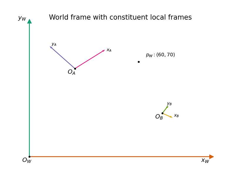
In the world frame, we can co-locate and relate points from different local systems together. See the below figure, which shows how a point p in the world frame can be related between multiple other frames, e.g. A and B. While we may only know the coordinates for a point in one frame, we eventually want to be able to express the coordinates of that point in other coordinate frames as well.
The world frame as shown in the figure above is useful as it demonstrates a coordinate frame in which we can reference the coordinates of OA and OB relative to the world frame. All coordinate systems are relative to some position; however, if OA and OB are only relative to themselves, we have no framework with which to relate them. So instead, we relate them within our world frame, which helps us visualize the differences between our coordinate systems A and B.
Relating two frames together
In the previous figure, we showed off two local frames A & B inside our world frame W. An important aspect in discussing coordinate frames is establishing a consistent notation in how we refer to coordinate frames and their relationships. Fortunately, mathematics comes to the rescue here as it provides some tools to help us derive a concise way of relating coordinate frames together.
Let's suppose we still have two coordinate frames we care about, namely coordinate frame A and coordinate frame B. We have a coordinate in frame A, pA, that we want to know the location of in frame B (i.e. we are searching for pB). We know that this point can exist in both frames, and therefore there is a functional transformation to convert to pB from pA. In mathematics, we express relations as a function:
We don't know what this function f is yet, but we will define it soon! It's enough to know that we are getting a point in coordinate frame B from coordinate frame A. The function f is what we typically call a transform. However, saying "the coordinate frame B from coordinate frame A transform" is a bit wordy. We tend to lean towards referring to this transform as the B from A transform, or B←A transform for brevity.
Notice the direction here is not A to B, but rather B from A. While this is a bit of a semantic distinction, the latter is preferred here because of how it is later expressed mathematically. We will eventually define a transformation matrix, ΓBA, that describes the transform f above. The superscript and subscript are conventionally written this way, denoting the B←A relationship. Keeping many coordinate frames consistent in your head can be difficult enough, so consistency in our notation and language will help us keep organized.
Now that we have a notation and some language to describe the relationship between two coordinate frames, we just need to understand what kinds of transforms we can apply between two coordinate frames. Fortunately, there's only 3 categories of transformations that we need to care about: translations, rotations, and scale!
Translation
Translations are the easiest type of coordinate transform to understand. In fact, we've already taken translation for granted when defining points in a Cartesian plane as offsets from the origin. Given two coordinate systems A and B, a translation between the two might look like this:
Mathematically, we might represent this as:
Pretty simple addition, which makes this type of transformation easy!
Rotation
Rotations are probably the most complex type of transform to deal with. These transforms are not fixed offsets like translations, but rather vary based on your distance from the origin of your coordinate frame. Given two coordinate frames A and B, a rotation might look like so:
In the 2D scenario like shown above, we only have a single plane (the XY-plane), so we only need to worry about a single rotation. Mathematically, we would represent this as:
This rotation matrix assumes that positive rotations are counter-clockwise. This is what is often referred to as the right-hand rule.
To get a point pB from pA we then do:
The matrix multiplication is a bit more involved this time, but remains quite straightforward. Fortunately this is the most difficult transformation to formulate, so we're almost there!
Scale
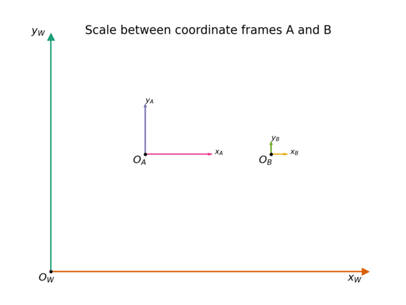
The final type of transformation we need to consider is scale. Consider the following diagram, similar to the ones we've shown thus far:
The two frames are again translated, but this is not important for what we're looking at here. Notice that the axes of A are a different length than the axes of B. This is a visual trick to demonstrate what scale transformations do between two coordinate frames. An example of a real-world scale issue might be a unit conversion. Namely, B might be in units of meters, while A is in units of millimeters. This scale difference will change the final results of any point pB relative to pA, by a multiplicative factor. If we have an isometric scale, we might represent this mathematically as:
Now, in this way, we are using a scalar value to represent an isometric scale across both x and y axes. This is not always the case, as sometimes our scale is not isometric. In robotics, we typically treat most of our sensors as having an isometric scale, but it is worth showing the mathematics for how one might generalize this if the scale in x (sx) is different from the scale in y (sy):
By utilizing this more general matrix equation over the scalar form above, it is easy to abstract between isometric scales (where sx = sy), and affine transforms. Fortunately it's often very easy to get away with assuming that our scale is isometric.
Putting it all together
Now that we know the three types of transforms, how do we put it all together? Any two coordinate frames A and B could have any number of translations, rotations, and scale factors between them. A transform in the general sense incorporates all three of these operations, and so we need a more formal way to represent them. Using our previous notation, we can formulate it as follows:
Keep in mind the order here:
- Rotation
- Scale
- Translation
With all the multiplications going on, this can get very confusing very quickly! Moreover, remembering the order every time can be pretty difficult. To make this more consistent, mathematicians and engineers often try to represent it as a single matrix multiplication. This way, the order is never confusing. We call this single matrix ΓBA. In plain English, we typically call this the B from A transformation matrix, or just the B←A transform. Unfortunately, however, you'll notice that not every operation in our above equation is a matrix multiplication, so the following doesn't work!
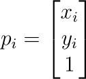
This would be fine for rotation and scale, but doesn't allow us to do anything about translations. Fortunately, we can work around this somewhat by leveraging a small trick of mathematics: increasing the dimensionality of our problem. If we change some of our definitions around, we can create a nuisance or dummy dimension that allows us to formulate ΓBA as:
Notice that our last dimension on each point remains equal to 1 on both sides of the transformation (this is our nuisance dimension)! Additionally, the last row of ΓBA is always zeros, except for the value in the bottom right corner of the matrix, which is also a 1!
If you want to learn more about the trick we're applying above, search for homogeneous coordinates or projective coordinates!
Try it for yourself with these Python functions! Find this and the code used to generate our above figures in our Tangram Visions Blog repository.
 Tangram-Vision
/
Tangram-Vision-Blog
Tangram-Vision
/
Tangram-Vision-Blog
Code pertaining to posts made on our official blog!
Tangram Visions Blog
This repo holds code to generate the assets used in the company blog for Tangram Vision! The main page of the blog can be found here.
See the README in each directory for instructions on installation, operation, and output.
Table of Contents
One to Many Sensors
- Code here
- 2020.11.30 post: One To Many Sensors, Part I
- 2020.12.04 post: One To Many Sensors, Part II
Coordinate Frames
- Code here
- 2021.01.21 post: Coordinate systems, and how to relate multiple coordinate frames together Part I
Exploring Ansible via Setting Up a WireGuard VPN
- Code here
- 2021.03.04 post: Exploring Ansible via Setting Up a WireGuard VPN
Color (Or Not)
- Code here
- 2021.03.?? post: Color (Or Not)
Contributing to this project
This is an open-source project; if you'd like to contribute a feature or adapt the code, feel free! We suggest you check out our contributing guidelines. After that, make…
What was it all for?
Knowing how to express relationships between coordinate frames both in plain English (I want the B←A or B from A transformation) and in mathematics (I want ΓBA) helps bridge the gap for how we relate sensors to each other. In a more concrete example, suppose we have two cameras: depth and color. We might want depth←color, so that we can fuse semantic information from the color camera with spatial information from the depth camera. Eventually, we want to then relate that information back to real world coordinates (e.g. I want world←depth).
Coordinate frames and coordinate systems are a key component to integrating multi-sensor frameworks into robotics and automation projects. Location is of the utmost importance, even more when we consider that many robotics sensors are spatial in nature. Becoming an expert in coordinate systems is a path towards a stable, fully-integrated sensor suite on-board your automated platform of choice.
While these can be fascinating challenges to solve while creating a multi-sensor-equipped system like a robot, they can also become unpredictably time consuming, which can delay product launches and feature updates. The Tangram Vision SDK includes tools and systems to make this kind of work more streamlined and predictable — and it's free to trial, too.
We hope you found this article helpful—if you've got any feedback, comments or questions, be sure to tweet at us!


Top comments (0)