Probability Distributions with Python: Discrete & Continuous

Context

There are several posts that could serve as context (as needed) for the concepts discuss in this post including these posts on:

• Conditional Probability
• Bayes' Theorem
• Bayes' Application & Code

Distributions

In this post, we'll cover probability distributions. This is a broad topic so we'll sample a few concepts to get a feel for it. Borrowing from the previous post, we'll chart our medical diagnostic outcomes.

You'll recall that each outcome is the combination of whether someone has a disease, P(D), or not, P(not D). Then, they're given a diagnostic test that returns positive, P(P) or negative, P(not P).

These are discrete outcomes so they can be represented with the probability mass function, as opposed to a probability density function, which represent a continuous distribution.

Let's take another hypothetical scenario of a city where 1 in 10 people have a disease and a diagnostic test has a True Positive of 95% and True Negative of 90%. The probability that a test-positive person actually having the disease is 46.50%.

Here's the code:

from random import random, seed

seed(0)
pop = 1000  # 1000 people
counts = {}
for i in range(pop):
    has_disease = i % 10 == 0  # one in 10 people have disease
    # assuming that every person gets tested regardless of any symptoms
    if has_disease:
        tests_positive = True       # True Positive  95%
        if random() < 0.05:
            tests_positive = False  # False Negative 5%
    else:
        tests_positive = False      # True Negative  90%
        if random() < 0.1:
            tests_positive = True   # False Positive 10%
    outcome = (has_disease, tests_positive)
    counts[outcome] = counts.get(outcome, 0) + 1

for (has_disease, tested_positive), n in counts.items():
    print('Has Disease: %6s, Test Positive: %6s, count: %d' %
          (has_disease, tested_positive, n))

n_positive = counts[(True, True)] + counts[(False, True)]
print('Number of people who tested positive:', n_positive)
print('Probability that a test-positive person actually has disease: %.2f' %
      (100.0 * counts[(True, True)] / n_positive),)

Given the probability that someone has the disease (1 in 10), also called the 'prior' in Bayesian terms. We modeled four scenarios where people were given a diagnostic test. Again, the big assumption here is that people get randomly tested. With the true positive and true negative rates stated above, here are the outcomes:

Probability Mass Function

Given these discrete events, we can chart a probability mass function, also known as discrete density function. We'll import pandas to help us create DataFrames and matplotlib to chart the probability mass function.

We first need to turn the counts of events into a DataFrame and change the column to item_counts. Then, we'll calculate the probability of each event by dividing the count by the total number of people in our hypothetical city (i.e., population: 1000).

Optional: Create another column with abbreviations for test outcome (i.e., "True True" becomes "TT"). We'll call this column item2.

import pandas as pd
import matplotlib.pyplot as plt

df = pd.DataFrame.from_dict(counts, orient='index')
df = df.rename(columns={0: 'item_counts'})
df['probability'] = df['item_counts']/1000
df['item2'] = ['TT', 'FF', 'FT', 'TF']

Here is the DataFrame we have so far:

You'll note that the numbers in the probability column adds up to 1.0 and that the item_counts numbers are the same as the count above when we had calculated the probability of a test-positive person actually having the disease.

We'll use a simple bar chart to chart out the diagnostic probabilities and this is how we'd visually represent the probability mass function - probabilities of each discrete event; each 'discrete event' is a conditional (e.g., probability that someone has a positive test, given that they have the disease - TT or probability that someone has a negative test, given that they don't have the disease - FF, and so on).

Here's the code:

df = pd.DataFrame.from_dict(counts, orient='index')
df = df.rename(columns={0: 'item_counts'})
df['probability'] = df['item_counts']/1000
df['item2'] = ['TT', 'FF', 'FT', 'TF']
plt.bar(df['item2'], df['probability'])
plt.title("Probability Mass Function")
plt.show()

Cumulative Distribution Function

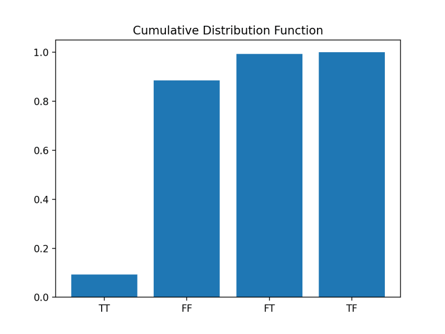
While the probability mass function can tell us the probability of each discrete event (i.e., TT, FF, FT, and TF) we can also represent the same information as a cumulative distribution function which allows us to see how the probability changes as we add events together.

The cumulative distribution function simply adds the probability from the previous row in a DataFrame in a cumulative fashion, like in the column probability2:

We use the cumsum() function to create the cumsum column which is simply adding the item_counts, with each successive row. When we create the corresponding probability column, probability2, it gets larger until we reach 1.0.

Here's the chart:

This chart tells us that the probability of getting both TT and FF (True, True = True Positive, and False, False = True Negative) is 88.6% which indicates that 11.4% (100 - 88.6) of the time, the diagnostic test will let us down.

Normal Distribution

More often than not, you'll be interested in continuous distributions and you can see better see how the cumulative distribution function works.

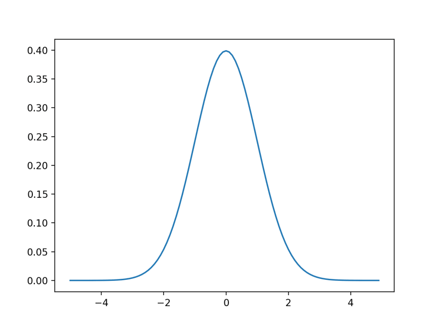
You're probably familiar with the bell shaped curve or the normal distribution, defined solely by its mean (mu) and standard deviation (sigma). If you have a standard normal distribution of probability values, the average would be 0 and the standard deviation would be 1.

Code:

import math
SQRT_TWO_PI = math.sqrt(2 * math.pi)

def normal_pdf(x: float, mu: float = 0, sigma: float = 1) -> float:
    return (math.exp(-(x-mu) ** 2 / 2 / sigma ** 2) / (SQRT_TWO_PI * sigma))

# plot
xs = [x / 10.0 for x in range(-50, 50)]
plt.plot(xs, [normal_pdf(x, sigma=1) for x in xs], '-', label='mu=0, sigma=1')
plt.show()

With the standard normal distribution curve, you see the average probability is around 0.4. But if you add up the area under the curve (i.e., all probabilities of every possible outcome), you would get 1.0, just like with the medical diagnostic example.

And if you split the bell in half, then flip over the left half, you'll (visually) get the cumulative distribution function:

Code:

import math

def normal_cdf(x: float, mu: float = 0, sigma: float = 1) -> float:
    return (1 + math.erf((x - mu) / math.sqrt(2) / sigma)) / 2

# plot
xs = [x / 10.0 for x in range(-50, 50)]
plt.plot(xs, [normal_cdf(x, sigma=1) for x in xs], '-', label='mu=0,sigma=1')

In both cases, the area under the curve for the standard normal distribution and the cumulative distribution function is 1.0, thus summing the probabilities of all events is one.

This post is part of my ongoing progress through Data Science from Scratch by Joel Grus:

For more content on data science, machine learning, R, Python, SQL and more, find me on Twitter.